HighlandMueller

Tonight, I will be putting out the text that I will use to address the City Council to argue for the ideas in AURA’s resolution.  One argument I will not be making, but that has been made by people whom I agree with most of the time and who I consider my friends, is that Highland is the same as Mueller.

I don’t understand the argument completely, but here are my reasons for not using it:

  1. It isn’t true.  At the most basic, simplistic level, Highland is a route that goes one place; Mueller is a route that goes someplace nearby, but different.  They share part of the same route, but not the whole thing.  AURA has emphasized that we should use actual, true facts in this process.  This isn’t an actual, true fact.
  2. It’s not clear why it matters.  There’s been a similar argument regarding the Red Line that Lakeline == Cedar Park.  In that case, the argument is that most of the passengers who take the Red Line from Lakeline station come from Cedar Park.  This matters because Cedar Park is not in the Cap Metro service area, so they are not paying taxes.  But Mueller is a part of Austin.  It’s not a priori obvious why having a route go to Mueller is bad.  My analysis says that Mueller is a less advantageous first route than Lamar or Riverside.  But then again, my analysis says the same about Highland, so bringing up Mueller just seems to confuse the issue.
  3. It makes Mueller sound evil, without explaining why.  I know a lot of people in the urbanist community are disappointed that Mueller didn’t become more urban, but most people in Austin don’t have some gut-level hatred for Mueller.  It’s a nice, growing neighborhood.  If you are implying that Highland is a stalking horse for Mueller, you either need to explain why that’s a bad thing or you sound like you just have an irrational hatred for one neighborhood.  Certainly, you can’t expect any politician to share in your concern.

Perhaps I’m missing something obvious.  But if so, maybe the argument needs to be fleshed out a bit better.  From my perspective, the fact that 2 years ago staff’s analysis chose Mueller and today’s staff analysis picks Highland, tells me that either: a) it’s a really good thing the public doesn’t just take staff’s word for granted because different staffs might come up with different answers, or b) projections can change rapidly, even in the span of just 2 years.

The Austin Precedent: Bus improvements block rail

The discussion on where Austin’s first urban rail route should run has switched tracks.  The Friday meeting of the mayor’s advisory group did not open with a discussion of the questions which have occupied this blog lately: which area of central Austin would best support an urban rail route (or vice-versa).  Instead, many advisory group members addressed emails from the public supporting studying a Lamar route by discussing what has been an elephant on the tracks: FTA funding for bus improvements.

Starting in January, Austin’s #1 bus route will see various improvements paid for by the FTA: longer buses, real-time information on bus location, wifi, longer spacing between stops.  Another bus route will see many of the same improvements a few months later.   As a frequent bus rider, I’m happy to see buses improve!  It’s a modest improvement–the buses will still get stuck in traffic through much of their routes.  But its benefits will not be limited to the #1 and #3 routes: the restricted-car lanes through downtown will eventually be used by most routes.  The heaviest costs of the real-time bus information system is setting up the system itself;  once the grant has paid for the upfront IT costs, Cap Metro will be able to expand it relatively inexpensively to the rest of the fleet.   Even the most expensive part of the system–the buses themselves–will save Cap Metro the cost of replacing the existing buses.  FTA is not funding *additional* buses along the #1 route, merely the routine cost of replacing buses, although the buses it’s replacing them with are nicer and more expensive than the buses Cap Metro would otherwise have bought.  Viewed this way, the FTA grant is less a massive upgrade to a couple of bus routes and more a clever way for the federal government to help pay for incremental improvements in Austin’s bus system, to be first deployed on Austin’s most popular bus route, the #1.

But was it too clever?  The argument at the mayor’s advisory group made was that FTA’s funding for these improvements would need to be paid back and reapplied for on a different route before the FTA would agree to upgrade a portion of the #1 bus to rail.  Furthermore, the FTA would not look kindly on Austin for applying for a larger, better rail project in an area they have already received funding and probably refuse to fund the rail.  Friend-of-the-blog Niran Babalola offers an interesting comment (via e-mail):

This example will be used around the country to demonstrate that investments in better buses push off rail for decades. This is counter to both the city of Austin’s interests (where MetroRapid in other corridors will probably be a good idea, but won’t be supported) and the FTA’s interests (who want cities to make bus investments until the money for rail appears, but will face more reluctance with this example).

So is it FTA policy that using FTA grants to improve your bus service endangers your ability to get funding for rail?  I don’t know; the most definitive piece of evidence on this question at the meeting was a sidebar conversation at a conference.  Julio believes this couldn’t possibly be right.   I hope an enterprising reporter can get the FTA to answer the question for us.  It’s a question with importance beyond Austin.

(In case it sounds like this is a novel worry; it’s not.  The furthest back I could find comment on this issue was Mike Dahmus’ blog posts from 2004, when the system was first proposed.)

Some more visualizations of Criteria and indices

Another day, another few new charts! 🙂

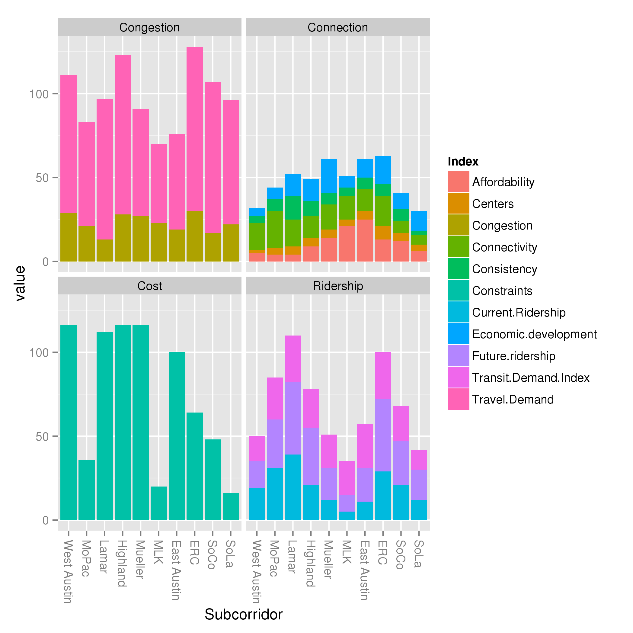
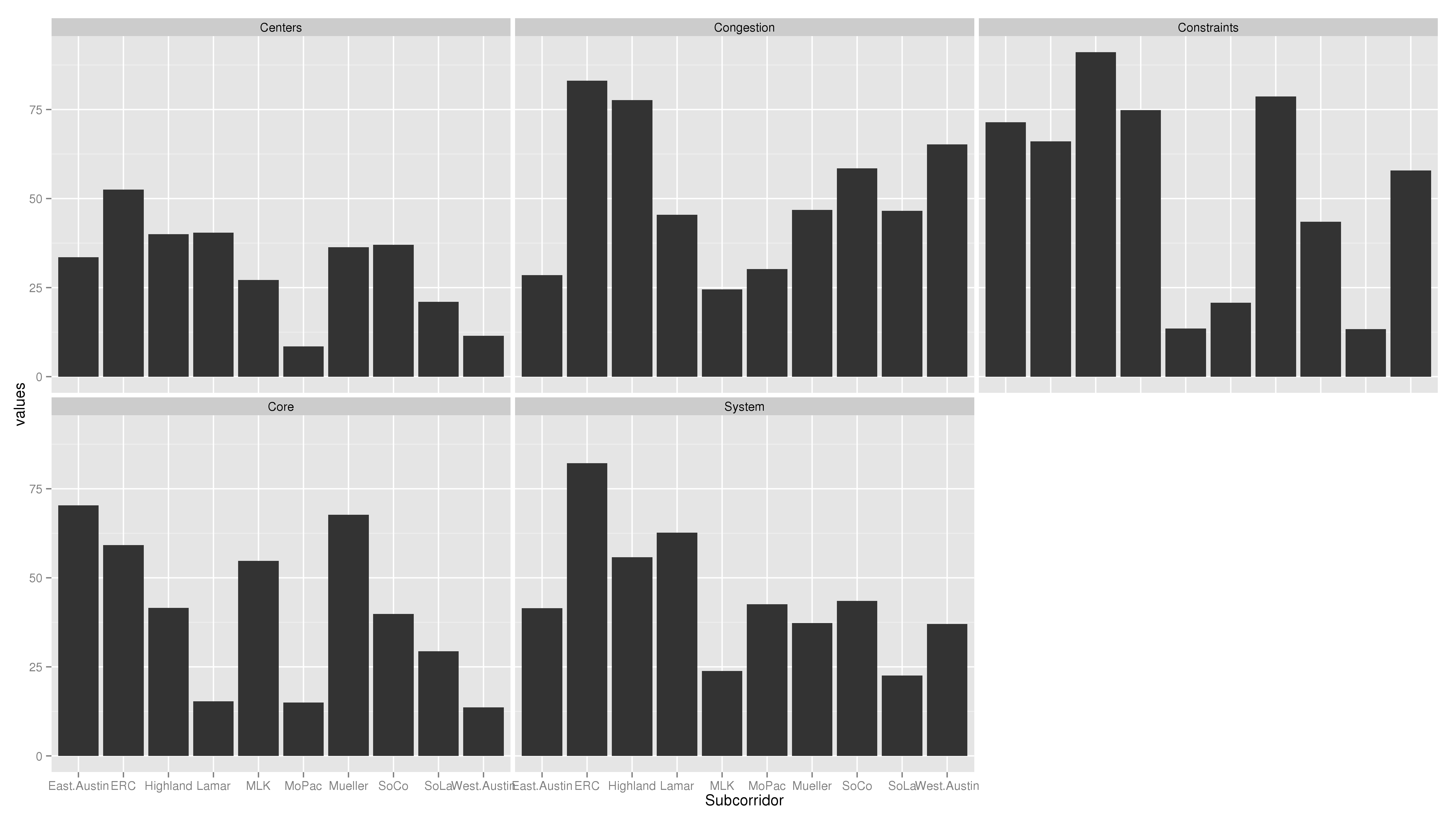
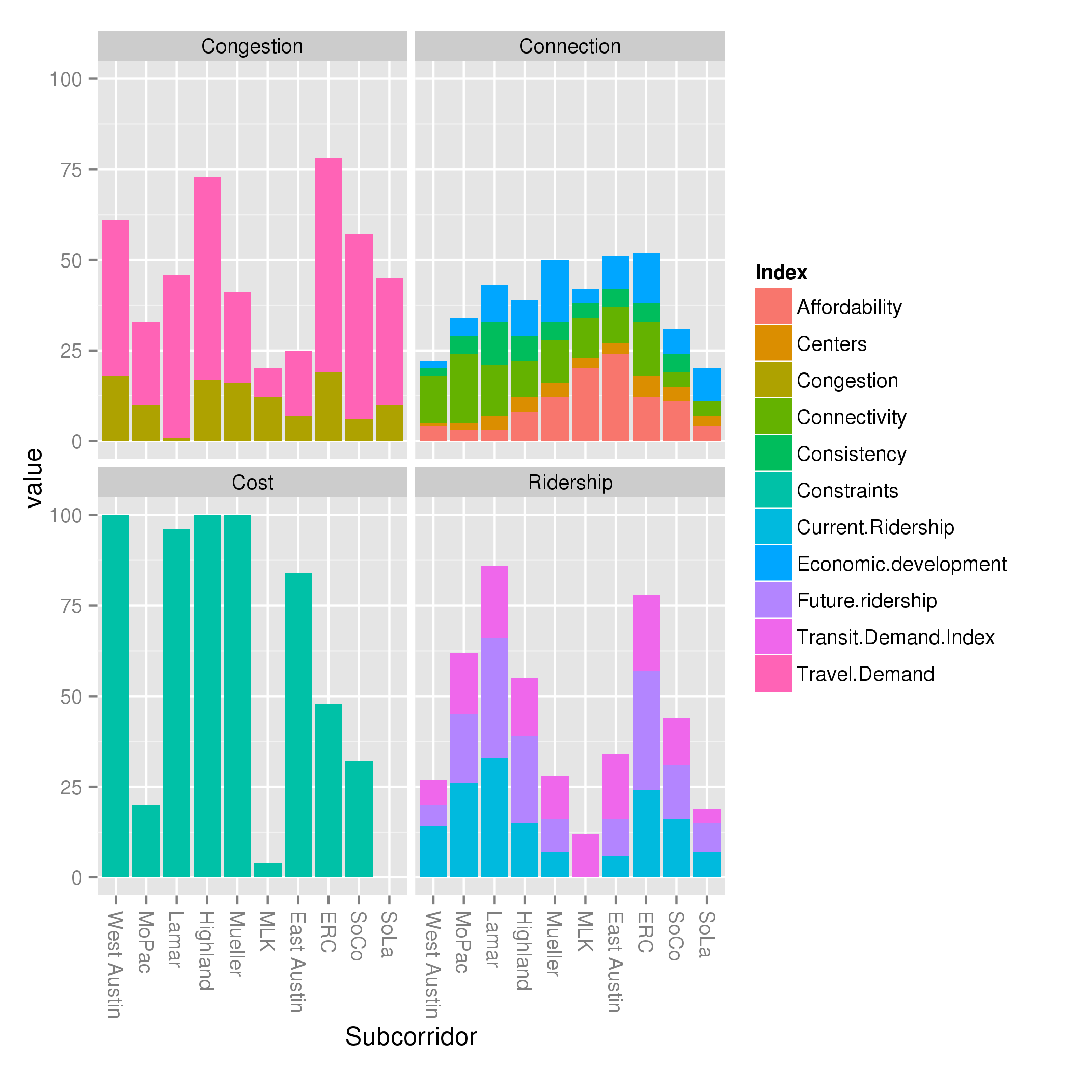
I have included 4 charts here.  When I presented the traditional, explanatory criteria, I created a visualization of how each subcorridor performed along each of these criteria.  But I began to wonder: which indices were driving the performance of each criteria?  So in these charts, I stack the contribution of the indices to the criteria:

Traditional criteria, normalized to min but not max

What can you learn from this?

  1. Weightings really matter.  Looking at the congestion chart, you can see the pink index ( Travel Demand Index) dominates the brownish one ( Congestion index ).  This is mostly because of the 5:2 weightings that Project Connect selected for those indices, and I maintained the same.
  2. If you track the orange “Affordability Index” at the base of the “Connections” criteria around the compass point, you can see it grow from a tiny amount in West Austin, peaking in East Austin, then start dropping again as it makes its way back around the compass.  This is a large driver of the “Connections” index, and is definitely making me question whether “Affordability” should be its own metric, separated from the rather junky “Centers” and “Consistency” metrics.
  3. The Ridership criteria is a more self-contained picture into one factor than the Connections criteria.  Although they both have multiple colors, picking a single color for the Ridership criteria will give you a similar picture as picking all 3: the 3 measures covary.  For the Connections criteria, this criteria may be useful for scoring, but not so much for gaining insight into characteristics of the subcorridors.

The next thing I began to wonder was about normalization.  As I discussed earlier today, Project Connect uses min-max normalization on all measures.  That is, it finds the minimum and maximum values any subcorridor score on a measure, then scale all the values from the minimum to the maximum.  I mentioned that I think 0 to maximum might be better, an idea I got from a coworker of mine.  The idea is that if you take, say, a measure like population density (measured in say, residents / acre), with 4 subcorridors scoring 65, 75, 95, 110 then normalize it along a min-max scale, you get the same values (0, .22, .67, 1) as if you have 4 subcorridors scoring 5, 15, 35, 50.   But in the first case, the subcorridors are within a factor of 2, while in the second case, the subcorridors are within a factor of 10!  Normalizing by max alone would result in scores of (.60, .68, .86, 1) versus scores of (0.1, 0.3, 0.7, 1).  A clear difference!

So I decided to rerun the whole analysis, normalizing by max rather than max and min.   That results in this chart:

Traditional criteria, normalized to max but not min

What did we learn?  A lot!  We can see that the congestion criterion, while showing dramatic differences above, shows very mild differences below.  Basically, all subcorridors are within a factor of 2 of one another.  Twice as much traffic is important, for sure.  But now look at the ridership criteria: the dramatic differences from one subcorridor to another maintained themselves.  While traffic might change as a factor of 2, ridership might change as a factor of 6!  Focusing solely on the blue “Current Ridership” index, we can see that MLK goes from non-existent (by definition, as the smallest subcorridor) in the far above chart, to a very small value in the near above chart.  It really is the case that Lamar and ERC score large multiples higher than MLK; that is not an artifact of min-max normalization like the large differences in congestion were.

Now, some caveats: some of this may be a result of the types of measures that went into each index.  I have not yet assessed that.

Also, some notes about these charts:

  • I have moved from showing the subcorridors in alphabetical order to using the order Project Connect prefers, around the compass from West Austin to MoPac to Lamar, etc.
  • I realize the colors are too similar.  Sorry.  Fixing that takes time and I wanted to get this out there tonight, before I go to bed.
  • In these charts, I have used the “Including West Campus in Lamar and MoPac” and “Eliminating negative weighting on present” data variants presented in this post.  I could rerun them for the other variants if there’s interest.

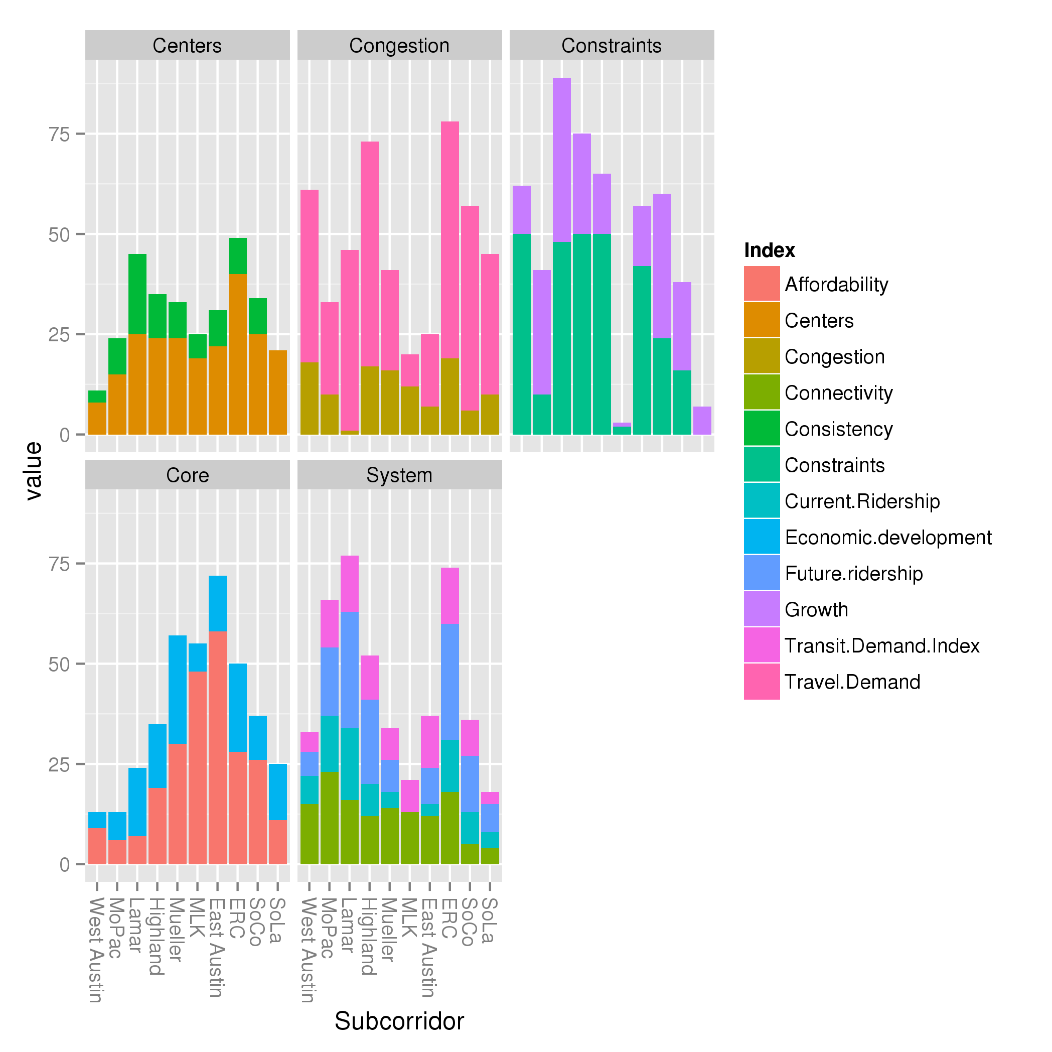
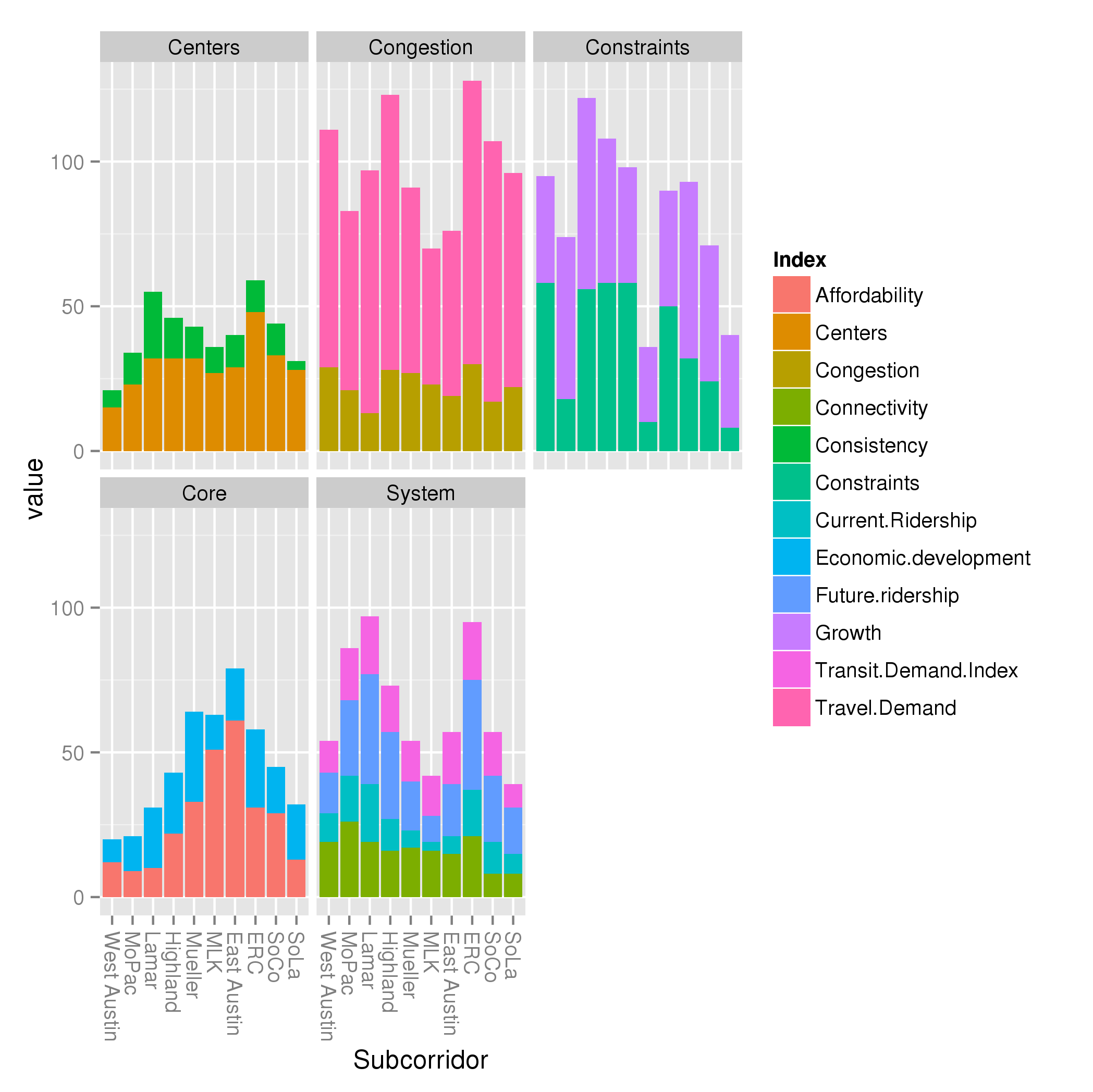
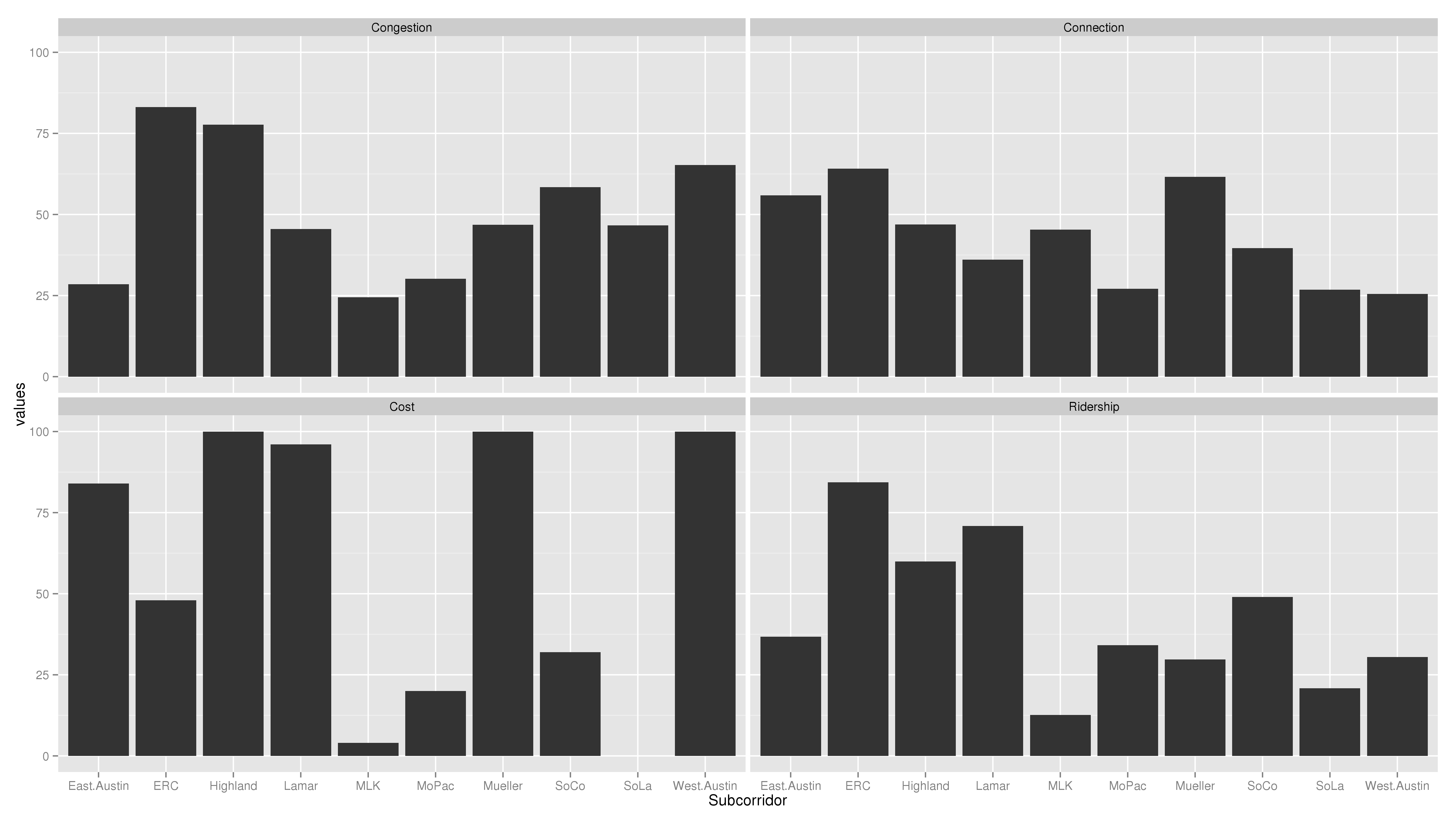
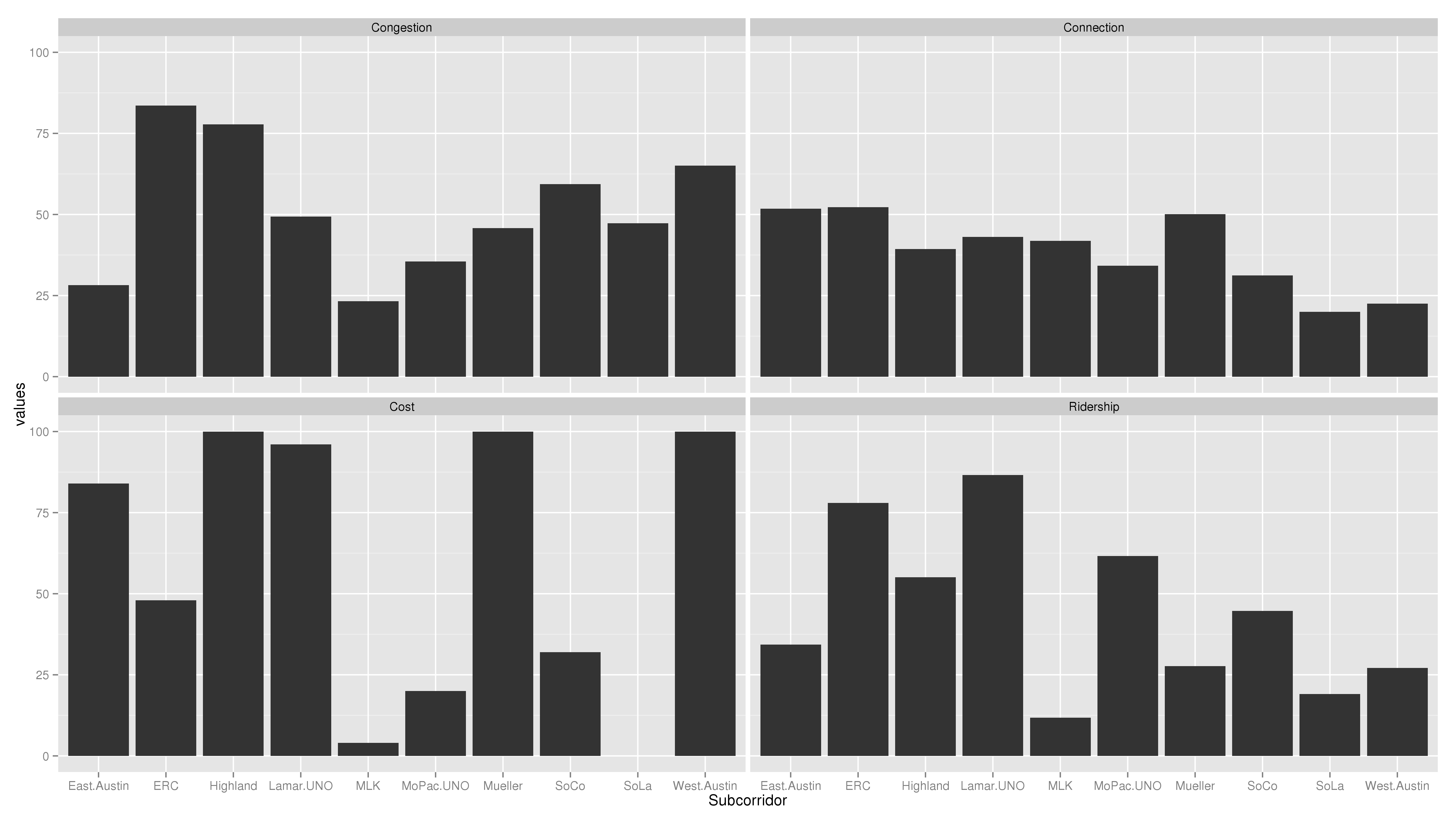
I also present Project Connect’s criteria, broken down by index (using min-max and max-only normalization):

Project Connect criteria, normalized to max and min
Project Connect criteria, normalized to max

What else do we learn from this?

  1. Constraints and growth is a ridiculous category for getting a handle on subcorridor performance.  These are two unrelated indices thrown together for no good reason.
  2. Similarly, the System criteria is mostly Ridership, but oddly diluted by throwing the unrelated Connectivity index in it.
  3. The “Core” metric is almost entirely affordability, along the familiar compass pointing East toward affordability.


Accurate charting and impact of West Campus

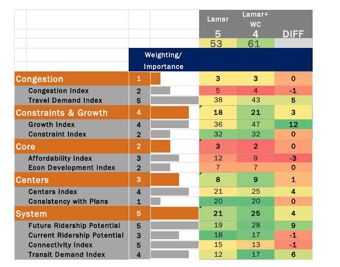
Project Connect has released a new FAQ.  In it, they show a comparison between Lamar with West Campus and without:
West Campus Comparison

Somehow, my numbers don’t add up the same as their numbers.  Any number of reasons could cause this discrepancy: I could have made an error in my hurry; their spreadsheet could not match the data they are using; I have found one such instance so far, but in that case, it was obvious.   A less obvious difference could easily have gone unnoticed.  They could’ve made an error, or they could be using a subtly different methodology than the one I believed to have reverse engineered.

However, the table they have produced above is at best sloppy.  At worst, it shows a lack of understanding of their own methodology and its implications.  Every single measure that Project Connect has produced has been normalized: that is, all the scores are rebalanced from 0 to 1, with the lowest-scoring subcorridor ranked 0, the highest 1, and the rest in between.

The “Diff” column in the above chart is not always meaningful, because each number in the “before” column and the “after” column may be set on different scales.  For a trivial example, take the “Consistency with Plans” index.  Lamar’s score without West Campus was 6.   6 was the highest score of the 10 subcorridors, so normalized, it becomes 1, and scaled up it becomes 20.  After adding in West Campus, Lamar’s score is 8.  This is of course still the highest of the 10 subcorridors, so normalized it also becomes 1, and scaled up it is still 20.  Lamar adds 0 to its score, as shown above.

However, scores only have meaning relative to one another.   East Riverside has a pre-normalized score of 4, a normalized score of 0.60, and a scaled-up score of 12.  After inclusion of West Campus in Lamar, it’s new normalized score is 0.43 or, scaled up, 9.  So, although Lamar’s “score” didn’t go up as a raw number, it did  improve by +3 relative to East Riverside.   Consistency with Plans is an unimportant, lowly-weighted index.  However, Future Ridership Potential is neither.  When including West Campus, Lamar scores highest on this metric as well.  That means that the “+9” difference is actually higher than +9, relative to the other subcorridors.

Unfortunately, these issues pervade the analysis.  Sloppy use of language in communications and sloppy charts such as the above don’t necessarily mean that their metrics chose the wrong subcorridor; it could just mean that they don’t take the time to write accurate communications.  However, it’s hard not to lose confidence in the choices that they made when they make elementary mistakes in the way that they present it.  Did they think through the implications of choosing to normalize from min to max, rather than what seems like the more obvious choice of 0 to max?  I would like to give them the benefit of the doubt that they had a good reason, but when I see sloppy charts like the one above it definitely shakes my confidence.

Update

So I set out to figure out where I disagree with Project Connect.  And, the first thing I find is data inconsistency between Project Connect’s online tool and the spreadsheet they released, on the very measure I discussed above:
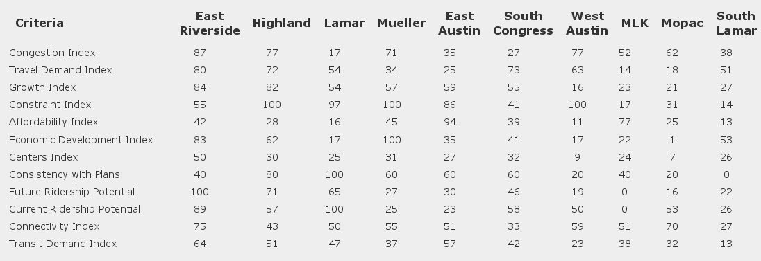
Raw Criteria from tool

Consistency Spreadsheet

Note the ERC’s score for consistency: 40 (0.4) on the online tool, and 0.6 in the spreadsheet.  This is the second such issue I’ve found; the first was an error in the spreadsheet.  Trying to reconcile difference between your calculations and theirs is nothing if not frustrating when there are data differences between two different versions of their own.  Identifying issues such as this are relatively easy in the Consistency criteria, as it consists of a single measure.  If there are errors in other measures, identifying them will be much more difficult.

Update 2

I misread the Project Connect FAQ.  My calculations are consistently very similar to theirs, and given the minor data issues like the ones above, I’m not surprised that they aren’t exactly equal.  Their wording on the effect of adding West Campus to Lamar is very squirrely: “Nevertheless, the overall impact improves the standing of the combined area by one position.”  From 3rd to 2nd.  From behind Highland to in front.   The same analysis as I found.  How they can repeatedly say adding West Campus doesn’t make a material difference and also say that it changes which the top two scoring corridors are is beyond me.

Update 3

Project Connect has updated their comparisons:

This is a step in the right direction, I think, though I’m still not completely sure what this means;  was this in a 11-way direct comparison?  Or was Lamar compared to Highland successively with and without Lamar?  (If so, there really need to be two columns for Highland: before and after.)   I did notice a disclaimer in a chart in Kyle’s presentation to CCAG that “numbers in columns cannot be compared to one another” which I appreciated.

But the basic message here is clear: inclusion or exclusion of West Campus makes a large impact on the final analysis.

A better visualization of effects of West Campus and time weighting

In my first glance, I showed that the Project Connect weightings resulted in different recommended subcorridors depending on whether you included West Campus in MoPac and Lamar, and whether you used negative weightings for present-day or used positive weightings for present-day, even if those weightings are smaller than those you use for the future.

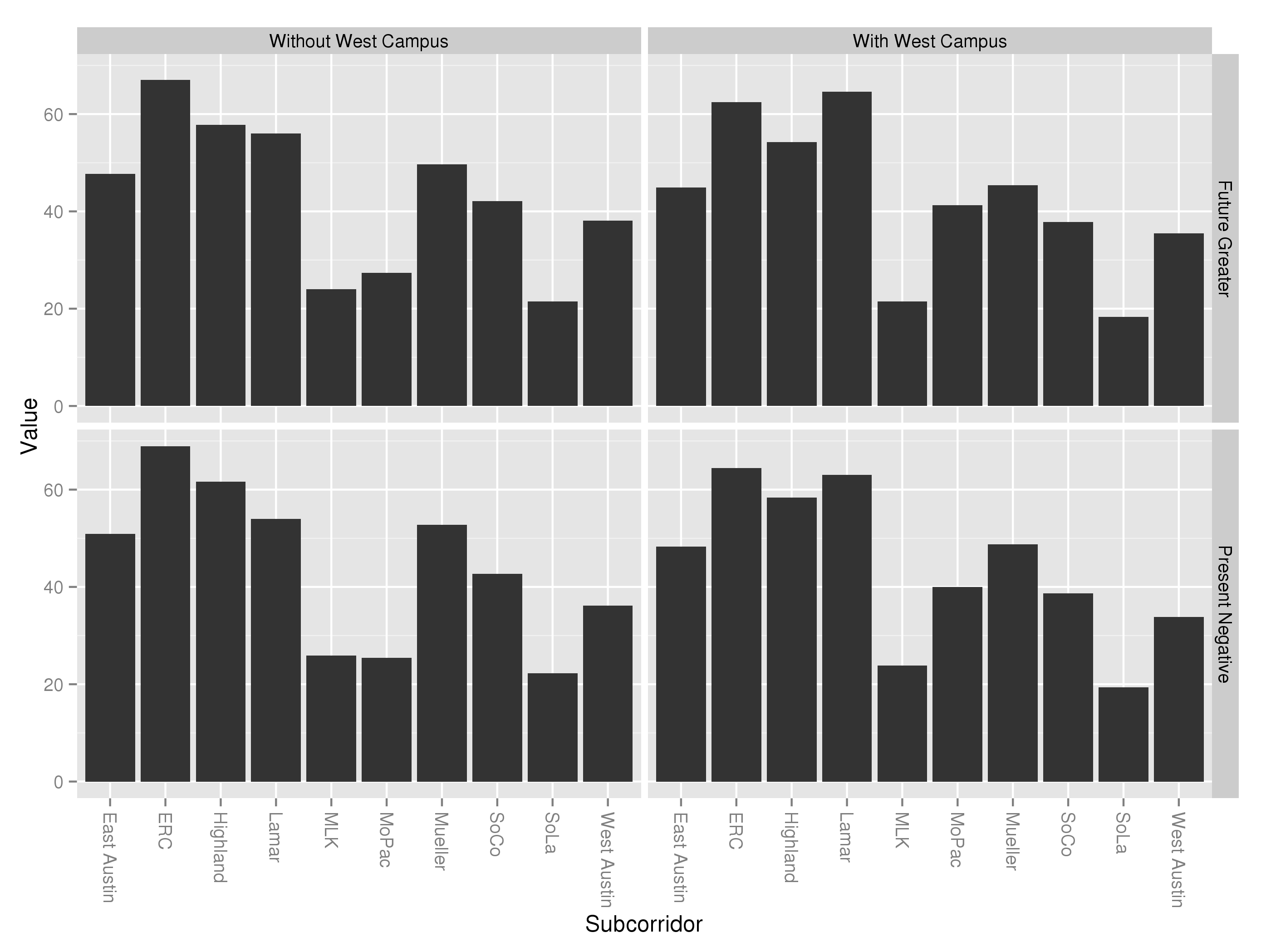
I have now put together a superior illustration for this effect here:Faceted Final Scores

As you can see, the choice to negatively weight present-day scores had a dramatic effect on the data excluding West Campus, pushing Highland and Lamar from a virtual tie (upper left) to Highland higher-rated (bottom left).  This is not surprising, as Project Connect’s methodology shows Highland as targeted for nearly 3.6% annual growth in population density.

When West Campus is factored into the mix, the effect continues.  However, this time the effect of the negative present-day weightings was smaller.  With a more balanced weighting (upper right), Lamar is the clear winner and Riverside second.  With the negative weightings, Lamar is second to Riverside’s first.  In both cases, Highland places third.

I still believe that Project Connect’s methodology for calculating the final score to be confusing and inferior to the more traditional weightings I employed here; one of the reasons for this is that their complications makes effects like these extraordinarily hard to understand at an intuitive level.  However, it is noteworthy that their data and methodology draw the same conclusions that mine did (Lamar and Riverside the top two subcorridors) when you include West Campus, and that it ranks Highland and Lamar as equal even excluding West Campus, if you just correct for the negative weightings of present-day data.

Breaking it down and building it back up

Yesterday, I started the process of replicating the Project Connect process, in order to understand the thinking behind their recommendation better.  I found in that process that making a few tweaks could change the outcome, but I didn’t gain a ton of insight into why the subcorridors scored as they did.  The point of using numbers to do analysis is not because numbers are impartial–numbers embody whatever biases the person using them brings to the table.  The point of using numbers to do analysis is to facilitate understanding–to tie empirical information to analytical categories.  So, I decided to break the final scores down by criteria and chart them.  BaseProjectConnect


As you can see from this chart…nothing.  Maybe you have a better understanding of Project Connect’s criteria than I do, but even months into this process, living and breathing this information, I have no intuitive understanding in my head of what these criteria mean, so these numbers aren’t really aiding in my understanding or decisionmaking.  So, I decided to come up with some criteria that answer some distinct questions of mine.

The questions I came up with (partially guided by what data is available from Project Connect) are as follows:

  1. Congestion How trafficky are the streets in this subcorridor?
  2. Connectivity A bit of a catch-all criteria measuring how closely this subcorridor aligns with other objectives of city planning.
  3. Cost How much will it cost to build a train in this subcorridor?
  4. Ridership Last, but obviously, not least, how many people can we reasonably expect to ride a train in this subcorridor?

So, I rejiggered the Project Connect indices to match these four new criteria.

  1. Congestion I used the same two indices that Project Connect did: Travel Demand Index and Congestion Index, at the same relative weighting (5:2).
  2. Connectivity I used five indices, all related to the question of city objectives.  I weighted the Affordability  index (which relates to legally-binding Affordable Housing), the Economic Development Index, and the Connectivity Index (which relates to sidewalk / bicycle / transit connectivity) all the same.  I gave half-weightings to the Centers Index and Consistency Index, both of which relate to how much transit is anticipated in official city plans, one using Imagine Austin criteria and the other using neighborhood plans.
  3. Cost I used a single index, the Constraint Index, which attempts to give a rough estimate of costs by counting costly things the train will have to cross: highways, lakes, creeks, etc.
  4. Ridership I used three indices to answer this question, all equally weighted: Future Ridership (an estimate of transit demand developed in Portland, Oregon based on projections of future residential, employment, and retail densities), Current Ridership (the same based on measured densities), and the Transit Demand Index (a homebrew formula similar to the other two, but including current ridership).

In putting this together, I used 11 of the 12 indices that Project Connect did.  I dropped the “Growth Index” as future projections are already embodied in indices such as the Future Ridership Index and the Congestion Index (which includes projected 2030 congestion measures).  Accounting for growth in its own index is what led Project Connect’s analysis odd results.  However, by organizing them along lines that answer clear questions in my head, I’m able to use them for easier analysis and not just scorekeeping.  This is what the chart looks like:

Answer my questions about each subcorridor, excluding West Campus from Lamar and MoPac, not correcting for "growth" issue.
Answer my questions about each subcorridor, excluding West Campus from Lamar and MoPac, not correcting for “growth” issue.

Now we’re getting somewhere!  This chart tells stories.  What I see here is that Riverside and Highland (including I-35, Airport, and Highland Mall) are the two most trafficky subcorridors.  Five subcorridors are relatively low-cost: East Austin, Highland, Lamar, Mueller, and West Austin.  Riverside is higher cost, and South Lamar would cost the most.  Which subcorridors interact well with other city priorities is pretty much a wash, with Riverside and Mueller scoring the highest.  Riverside and Lamar would have the highest ridership, with Highland establishing itself in a solid third.

Now, another view, this time with West Campus included in the Lamar and MoPac subcorridors:

Answering my questions, this time with West Campus included.

This tells another story: both the Lamar and MoPac subcorridors have seen large increases in ridership.  In this view, it’s clear that there are two major routes for high transit ridership: Lamar and Riverside, in that order.  Highland has decent ridership, but even building the low-ridership MoPac subcorridor would have higher ridership, just because it would go through the super-high-ridership West Campus neighborhood.

Analysis

Based on these charts, Lamar and Riverside seem frankly head-and-shoulders above the rest of the subcorridors.  I could construct “final scores” for each subcorridor, but why bother?  The key reason I say that lies in the interpretation of the “Congestion” Question.  The question that the Congestion chart answers is not: how much congestion would be relieved in this subcorridor if we built a train here?  The question is: how trafficky is this subcorridor?  Put another way, congestion is both a blessing and a curse: it shows that there is high transportation demand, but it also shows strong automobile orientation of the infrastructure.  Between two subcorridors which promise high ridership–now and in the future–and two subcorridors which promise to be congested–now and in the future–I opt to send the train where the people will ride it.

Caveats

This analysis is only as good as the information that went into it.  As Julio pointed out, for the future criteria, there’s reason to doubt that is true.  In addition, though I have rejiggered the criteria to more closely answer the types of questions needed to analyze the subcorridors, I haven’t yet dug into the individual indices much to see if the measures they use to answer their sub-questions make sense.

Again, this was coded in R and code will be furnished upon request.

A first glance at Project Connect data

Project Connect has generously shared most of its intermediate findings. I took the opportunity to look over some of their work over the last couple days. It’s a complicated task, as they included a vast number of measures, far more than truly needed for the task. In deciding how to report its results, AURA has disagreed with Project Connect on a number of areas.  Some of these include:

  • After it began its analysis, Project Connect decided to change the definition of the subcorridors, such that the population-rich, transit-heavy West Campus was no longer included in the Lamar and MoPac subcorridors.
  • Project Connect not only overweights future measures compared to present measures, it actually underweights present measures so much so that, in many areas, a subcorridor projected to have more congestion or density in 2010 and 2030 may be ranked lower than a subcorridor with less congestion or density in both time periods, just because the weaker subcorridor is projected to add more people.  Put another way, in their methodology, two birds in hand are worth one in the bush.  See my previous post for details.
  • Project Connect included I-35 information in the congestion figures for many of the subcorridors, without regard to whether a more significant fraction of highway drivers are nonlocal and less likely to get out and use a train than locals.

I have rerun Project Connect’s scoring methodology to account for each of these issues.  I found that highway data was not important for congestion measures, and resulted in similar measurements to Project Connect’s.  However, both the hyper-overweighting of the future and the exclusion of West Campus data were significant issues with Project Connect’s methodology, masking the strength of the Lamar subcorridor to the benefit of the Highland subcorridor.  Merely removing the hyperoverweighting of the future, but keeping the future weighted stronger than the present, and including West Campus in the analysis, results in the intuitive result that the Lamar subcorridor is ranked highest, East Riverside second, and Highland, Mueller, and East Austin lumped together.

I’m not going to say that these are the final results I believe in yet.  It wasn’t until I dug into Project Connect’s methodology that I noticed some of the strange preferences they embody, such as the hyperoverweighting of the future compared to the present.  Most likely, using a bottom-up method of selecting a few of the most salient measures from their analysis will be more productive in making a final selection, something that Julio has started very ably.

However, my analysis here makes one thing clear: the repeated assertion that the numbers point to the same conclusion any which way you dice them is nonsense.  It actually takes torturing the data quite a bit to result in the particular recommendation that they did: merely failing to hyperoverweight the future to the present or failing to exclude West Campus from the analysis changes the results materially.

Methodology

I downloaded the data from Project Connect.  I used the measure weightings from this document and the index weightings from this document.  I validated my intermediate results by using the weightings from the survey.  For the West Campus data, I used the “West Campus” tab with only one change: I set the “consistency” measure for MoPac and Lamar subcorridors to 4 and 8–adding in the “2” result for West Campus with the original “2” and “6” results for the two subcorridors, in place of the 0’s in the spreadsheet, which I believe was in error.  For the “overweighted future” scores, I set the weightings for all measures that were “increase from 2010 to 2030” to “0” and left the 2030 and 2010 weightings alone.  (2030 was already overweighted compared to the present; it was the increase that was responsible for the hyperoverweighting.)

I will continue to try to do analysis on this so that we can understand a clear story about what the data means, and not just “what are the final results.”  If you have particular questions you’d like me to answer, please let me know in the comments or on twitter or any which other way you know to reach me.  The code is in R and is available upon request.

A little oddity in Project Connect Evaluation Criteria

I was reviewing the Project Connect evaluation criteria, when I noticed a bit of an oddity:

Lane miles contribution

In examining congested lane miles, 2010 congestion data counts 3%, 2030 congestion projections count 5%, and the difference between the two counts 4%.  Making the difference between the projections and the real-world data count more than the real-world data means that not only does 2030 count more than 2010 data, but, given two subcorridors with the same 2030 projections, the one with less congestion in 2010 is measured as worse.

Note: The columns 2010 and 2030 are measured in %’s.  The weighted columns consist of the previous column, multiplied through by the percentage it counts toward the total and then by 100 for readability.

Name 2010 Weighted Increase Weighted 2030 Weighted Total
A 3 9 17 68 20 80 157
B 17 51 3 12 20 80 143

To repeat, Subcorridor A and B are tied in the 2030 metric, Subcorridor B was measured as more congested in 2010, but in total,  Subcorridor A is measured as more congested.  You could even construct examples where A was more congested than B in 2010 and 2030, but B is measured as more congested overall:

Name 2010 Weighted Increase Weighted 2030 Weighted Total
A 26 78 5 20 31 155 253
B 5 15 25 100 30 150 265

To repeat, in this example, Subcorridor A is more congested in both 2010 and 2030, but the Project Connect evaluation criteria measures Subcorridor B as overall more congested because it shows a large increase.  I could potentially construct a rationale for this: perhaps the increase between 2010 and 2030 represents a trend that will continue out into the future beyond 2030.  But this would not be a recommended use of the model; there are reasons we don’t use simple linear extrapolation in the model in the first place.  This odd situation could be avoided by simply not including the increase as a metric at all.

What effect did this have overall on the results?  I’m not sure; the individual scores for each subcorridor have not yet been released.  I really can’t predict how the scores would’ve been affected.  I will be speaking with Project Connect soon and hope to hear their rationale.

Update: The original Example 2 was messed up.  This version is fixed (I hope!).  Update 2: Improved readability by expressing things as percentages rather than decimals.

Update 3: For a little more discussion of this, you could break up the 2030 projections into two components: Base (2010) + Increase.

If you consider just 2010 data (as FTA suggests), you are going 100% for Base, 0% for Increase.

If you consider half 2010 data and half 2030 projections  (as FTA allows), you are going 75% for Base and 25% for Increase.

If you consider just 2030 projections, you are going 50% for Base and 50% for Increase.

But using Project Connect’s weightings here, you are weighted at 46% Base, 54% Increase, even more weighting on the increase than if you had just used the projections themselves.

The exact same issue applies to the “Growth Index”, in which a 50%-50% weighting between Increase and Future yields a 25% weighting for the Base and a 75% weighting for the Increase, the flip weighting of what the FTA suggests.